Microsoft Excel (hereinafter simply - Excel) is a program for performing calculations and managing so-called spreadsheets.
Excel allows you to perform complex calculations that can use data located in different areas of the spreadsheet and linked together by a certain dependency. To perform such calculations in Excel, it is possible to enter various formulas into table cells. Excel performs the calculation and displays the result in the formula cell.
An important feature of using a spreadsheet is the automatic recalculation of results when cell values change. Excel can also create and update graphs based on the numbers you enter.
A cell address in spreadsheets consists of the column name followed by the row number, for example C15.
To write formulas, use cell addresses and arithmetic operations signs (+, -, *, /, ^). The formula begins with =.
Excel provides standard functions that can be used in formulas. These are mathematical, logical, text, financial and other functions. However, in the exam you may encounter only the simplest functions: COUNT (number of non-empty cells), SUM (sum), AVERAGE (average value), MIN (minimum value), MAX (maximum value).
The cell range is designated as follows: A1:D4 (all cells of the rectangle from A1 to D4.
Cell addresses can be relative, absolute, or mixed.
They behave differently when copying a formula from cell to cell.
Relative addressing:
If in cell B2 we write the formula =D1+3, then the table will perceive this as “take the value of the cell two to the right and one above the current one, and add 3 to it.”
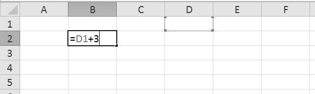
Those. address D1 is perceived by the table as a position relative to the cell where the formula is entered. This address is called relative. When copying such a formula to another cell, the table will automatically recalculate the address relative to the new location of the formula:

Absolute addressing:
If we don’t need the address to be recalculated when copying the formula, we can “fix” it in the formula - put a $ sign in front of the letter and cell index: =$D$1+3. This address is called absolute. This formula will not change when copied:

Mixed addressing:
If we want, when copying a formula, only the cell index is automatically recalculated, for example, and the letter remains unchanged, we can “fix” only the letter in the formula (or vice versa): =$D1+3. This address is called mixed. When copying a formula, only the index in the cell address will change:

Spreadsheets. Copying formulas.
Example 1.
Cell C2 contains the formula =$E$3+D2. What form will the formula take after cell C2 is copied to cell B1?
1) =$E$3+C1 2) =$D$3+D2 3) =$E$3+E3 4) =$F$4+D2
Solution:
The location of the formula changes from C2 to B1, i.e. the formula is shifted one cell to the left and one cell up (the letter “decreases” by one and the index decreases by one). This means that all relative addresses will also change, but absolute ones (fixed with the $ sign) will remain unchanged:
=$E$3+С1.
Answer: 1
Example 2.
The formula is written in cell B11 of the spreadsheet. This formula was copied into cell A10. As a result, the value in cell A10 is calculated using the formula x-Zu, Where X- the value in cell C22, and at- value in cell D22. Indicate what formula might have been written in cell B11.
1) =C22-3*D22 2) =D$22-3*$D23 3) =C$22-3*D$22 4) =$C22-3*$D22
Solution:
Let's analyze each formula in turn:
The location of the formula changes from B11 to A10, i.e. the letter "decreases" by 1 and the index decreases by 1.
Then when copying the formulas will change as follows:
The problem conditions correspond to formula 2).
Answer: 2
Spreadsheets. Determining the meaning of a formula.
Example 3.
Given is a fragment of a spreadsheet:
The formula is entered in cell D1 =$A$1*B1+C2, and then copied to cell D2. What value will appear in cell D2 as a result?
1) 10 2) 14 3) 16 4) 24
Solution:
The location of the formula changes from D1 to D2, i.e. the letter does not change, but the index increases by 1.
So the formula will take the form: =$A$1*B2+C3. Let's substitute the numerical values of the cells into the formula: 1*5+9=14. The correct answer is listed at number 2.
Answer: 2
Example 4.
In a spreadsheet the value of a formula =AVERAGE(A6: C6) equals ( -2 ). What is the value of the formula =SUM(A6: D6) , if the value of cell D6 is 5?
1) 1 2) -1 3) -3 4) 7
Solution:

By definition of average:
AVERAGE(A6: C6) = SUM(A6:C6)/3 = -2
Means, SUM(A6:C6) = -6
SUM(A6: D6) = SUM(A6:C6)+D6 = -6+5 = -1
Answer: 2
Spreadsheets and charts.
Example 5.
A fragment of a spreadsheet in formula display mode is given.

After performing the calculations, a diagram was built using the values of the range A1:D1. Indicate the resulting diagram:
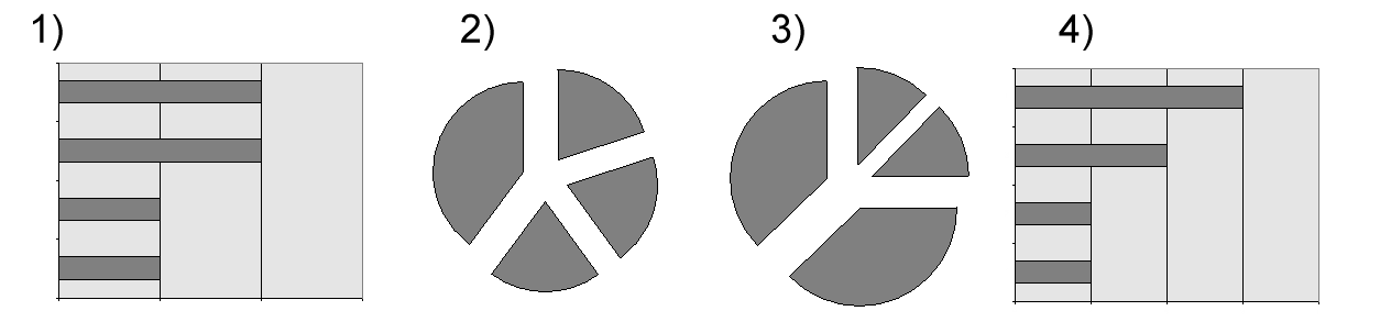
Solution:
Let's calculate the values of cells A1:D1 using formulas.
Diagram 3 corresponds to these data.
Answer: 3
7.1 (ege.yandex.ru-1) A fragment of a spreadsheet is given:
Solution:
From the second equation we find: C1=3. Let's check that this value is also suitable for the first equation:
2*(4-3) = 2*1 =2
Answer: 3
7.2 (ege.yandex.ru-2) A fragment of a spreadsheet is given:
What integer must be written in cell C1 so that the pie chart drawn for the range A2:C2 matches the figure? It is known that all values of the range on which the diagram is constructed have the same sign.
Solution: The diagram is built using the values of three cells: A2, B2, C2. From the pie chart you can see that these values are related as 1:1:1. Since the values of cells A1 and B1 are known, let's fill the range A2:C2 with values instead of formulas (where possible):
Since the values in all cells of the range A2:C2 must be equal, then for the value C1 we obtain two equations:
From the second equation we find: C1=2. Let's check that this value is also suitable for the first equation:
Answer: 2
7.3 (ege.yandex.ru-3) A fragment of a spreadsheet is given:
What integer must be written in cell B1 so that the pie chart drawn for the range A2:C2 matches the figure? It is known that all values of the range on which the diagram is constructed have the same sign.
Solution 1: The diagram is built using the values of three cells: A2, B2, C2. From the pie chart you can see that these values correlate as 2:1:1, while it is not known which cell corresponds to which sector of the chart. Let's simplify the formulas, given that we know the value for cell A1:
From the formula in cell C2, you can see that the values of B2 and C2 are different. Therefore A2 = B2. This gives us the equation for B1:
3-B1 = (3*B1+3)/3
Let's solve the equation.
Answer: 1
Solution 2 (similar reasoning, a little shorter) : The diagram is built using the values of three cells: A2, B2, C2. From the pie chart you can see that these values correlate as 2:1:1, while it is not known which cell corresponds to which sector of the chart. From the formula in cell C2, you can see that the values of B2 and C2 are different. Therefore A2 = B2. Considering that C1 = A1+1 = 2+1 =3, we obtain the equation for B1
3-B1 = (3*B1+3)/3
Let's solve the equation.
Let's check ourselves - find the values in all the cells of the table
Answer: 1
7.4 (ege.yandex.ru-4) A fragment of a spreadsheet is given:
What integer must be written in cell A1 so that the pie chart drawn for the range A2:C2 matches the figure? It is known that all values of the range on which the diagram is constructed have the same sign.
Solution: The diagram is built using the values of three cells: A2, B2, C2. From the pie chart it can be seen that these values correlate as X: 1: 1, where X is approximately equal to 4. However, it is not known which cell corresponds to which sector of the diagram. Let's simplify the formulas in the table, taking into account that C1=2. We get:
Since B2 > C2, then A2=C2 must be satisfied. We get:
whence A1=7.
Answer: 7
7.5 (ege.yandex.ru-5) A fragment of a spreadsheet is given:
What integer must be written in cells B1 so that the pie chart drawn for the range A2:C2 matches the figure? It is known that all values of the range on which the diagram is constructed have the same sign.
Solution: The diagram is built using the values of three cells: A2, B2, C2. From the pie chart you can see that these values are in a 2:1:1 ratio. That is, one of the values (the larger one) differs from the others, and the two smaller values are equal to each other. In this case, it is not known which cell corresponds to which sector of the diagram. Let's simplify the formulas in the table, taking into account one hundred A1=4. We get:
Let's look at the formula =B2+4 in cell C2. You can see that the value in cell C2 is 4 greater than the value in cell B2. In other words, the values in cells B2 and C2 are different, with C2 > B2. This means C2 is the larger of the three numbers, and A2 = B2 is the two smaller ones. Moreover, the diagram shows that C2 is twice as large as A2 and B2. Therefore done:
This gives us a system of two equations to determine the values of B1 and C1:
B1-C1+4 = 2*(B1-C1)
From the 1st equation: B1 = 5*C1. Substitute into the 2nd equation:
5*C1 – C1 + 4 = 2*(5*C1-C1)
Therefore, B1=5. We do a check - we calculate the values for all cells:
For this task you can get 1 point on the Unified State Exam in 2020
Task 7 of the Unified State Exam in computer science is devoted to the analysis of diagrams and spreadsheets. When solving this test, you will have to, for example, determine the values of formulas based on certain parameters. A typical question for this option is: “If the arithmetic mean of four values in the table is 5, then what is the sum of the first three cells if the fourth cell contains the number 6 and there are no empty cells in the table.”
In other versions of task 7 of the Unified State Exam in computer science, the student will be asked to make a diagram using the given data. For example, you are given the compositions of two substances with indications of the mass fractions of their components. It is required to determine the ratio of these elements in an alloy of two substances and find the correct one among the presented diagrams. The ticket may also contain tasks to determine the total income of each family member over a period of time, the volume of the harvest for each variety of cucumbers, the number of schoolchildren participating in subjects in different regions of Russia, the increase in prices of some goods as a percentage relative to the beginning of the year .
Problems of type A7 in computer science imply knowledge technologies for processing information in spreadsheets. Even more specifically - absolute and relative addressing.
As an example, consider solution to problem A7, consider solution A7 demo version of the Unified State Exam 2013 in computer science:
A fragment of a spreadsheet is given.
| A | B | C | D | |
| 1 | 1 | 2 | 3 | |
| 2 | 5 | 4 | = $A$2 + B$3 | |
| 3 | 6 | 7 | = A3 + B3 |
What will the value of cell D1 be equal to if you copy the formula from
cells C2?
Note: The $ sign denotes absolute addressing.
1)18 2)12 3)14 4)17
Solution:
Let's look at the contents of cell C2. It contains a formula that uses two cells, with cell references completely absolute($A$2) or partially absolute(B$3). When copying from cell C2 to cell D1, the address of cell $A$2 will remain the same, since its address is specified absolutely. The address of cell B$3 is set partially absolute - when copying, the row number will not change, but the column will change. When copying from column C to column D, the address of cell B$3 will change by 1 and become C$3. As a result, after copying, cell D1 will contain the formula = $A$2 + C$3. We know the contents of cell A2 - it is equal to 5. The contents of cell C3 need to be calculated: A3 + B3 = 6 + 7 = 13. We obtain that the value of cell D1 will be equal to 5 + 13 = 18. Correct answer 1.
As a reinforcement Let's solve problem A7 of the demo version of the Unified State Exam 2012 in computer science:
Cell B4 of the spreadsheet contains the formula = $C3*2. What will the formula look like after cell B4 is copied to cell B6?
Note: The $ sign is used to indicate absolute addressing.
1) = $C5 *4 2) = $C5 *2 3) = $C3 *4 4) = $C1 *2
Solution:
In the formula = $C3 * 2, the addressing of cell $C3 is partially absolute - when copying, only the row number changes (since it is preceded by a $ sign), and the column remains unchanged. When copying from cell B4 to cell B6, the line number will increase by 2, therefore the address of cell $C3 will turn into $C5. As a result, cell B6 will contain the formula = $C5 * 2. Correct answer 2.
Analysis of task 7 of the Unified State Exam 2017 in computer science from the demo version project. This is a task of a basic level of difficulty. Approximate time to complete the task is 3 minutes.
Content elements tested: knowledge of technology for processing information in spreadsheets and methods of visualizing data using charts and graphs. Content elements tested on the Unified State Exam: Mathematical processing of statistical data. Using tools for solving statistical and computational-graphical problems.
A fragment of a spreadsheet is given. A formula was copied from cell A2 to cell B3. When copying, the cell addresses in the formula automatically changed. Write down the numerical value of the formula in cell B3 in your answer.
Note: The $ sign denotes absolute addressing.
Answer: ________
Our formula =C$2+D$3 in a cell A2 contains two mixed links.
- in the first C$2- the address of line 2 does not change when copying
- in the second D$3- the address of line 3 does not change when copying
Our formula =C$2+D$3 was copied from a cell A2 to cell B3.
— moved one column to the right (increased by one column)
— moved one line down (increased by one line)
Therefore, after copying the formula =C$2+D$3, will take the form =D$2+E$3.

Evaluating this expression gives the following result: 70+5=75 .


